Affinity propagation in R

Today we’ll have a closer look on the fundamentals of affinity propagation and how to run this kind of clustering algorithm in the R programming language. Affinity propagation is based on the message-passing principle and requires no prior definition of the number of clusters. Affinity propagation scales well with the size of data points. Moreover, this clustering algorithm does not require symmetric similarity matrices [i.e., ] and can be applied to problems where the triangle equality for the similarities [] is not met.

Affinity propagation uses 4 matrices:

• similarity matrix
• responsibility matrix
• availability matrix
• criterion matrix

After running the algorithm, so-called exemplars are identified, that are data points that are representative of the clusters, this means: objects that end up with a specific exemplar are clustered together. Within the data set, all data points are equally suitable to represent an exemplar and when initializing, the preferences should be set to a common value. According to Frey & Dueck (2007), for generating a moderate number of clusters, the shared value should be set to the median of the input similarities, while for a low number of clusters, it should be set to their minimum value. Ultimately, the number of the resulting exemplars (corresponding to the clusters) is governed by the values of the input preferences and the message-passing method.

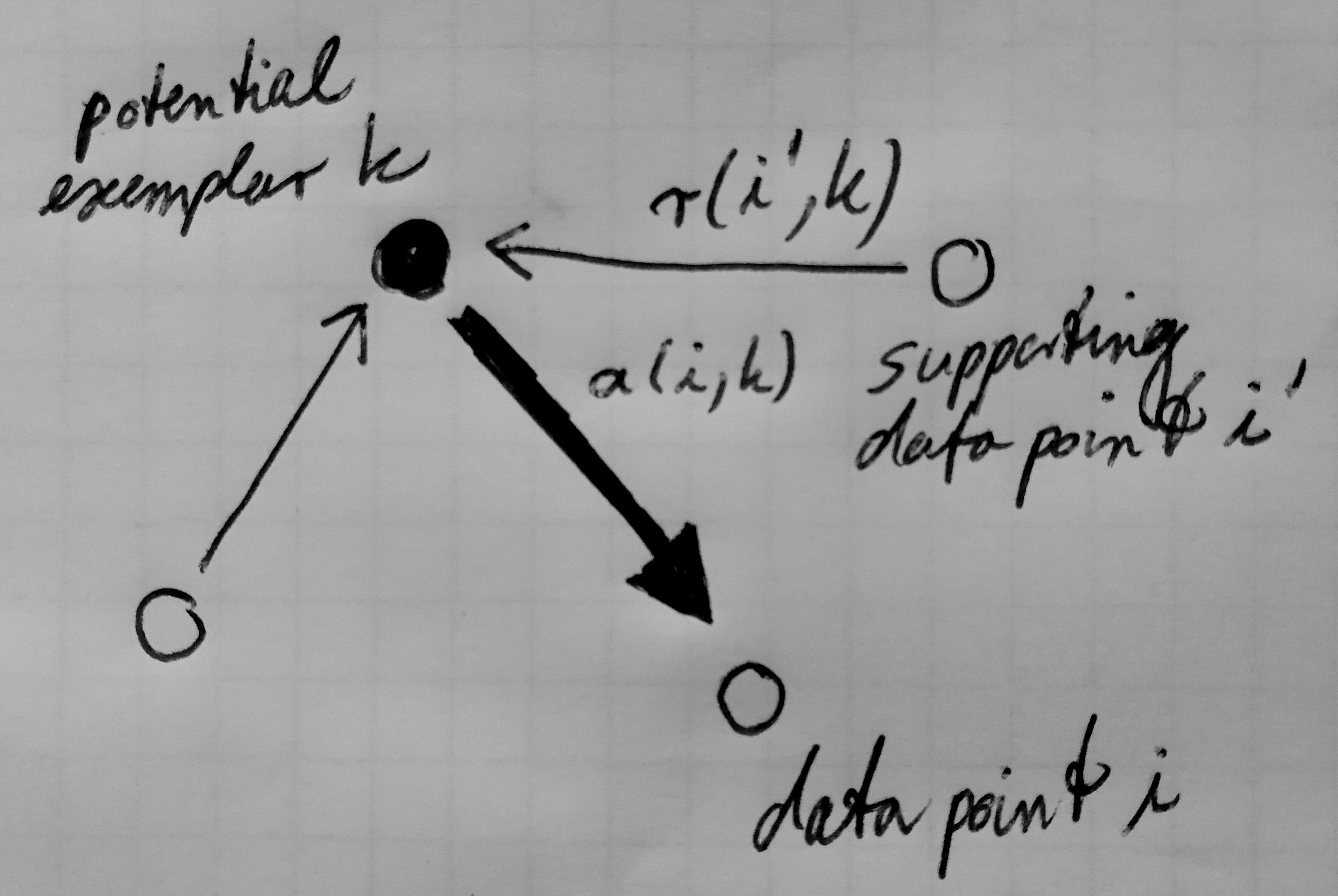
In the following, we will quickly go through the two major kinds of messages, which are exchanged between the data points of the data set, that are fundamental to affinity propagation clustering. One message, called the responsibility r(i,k), is sent from a data point i to a candidate exemplar point k. The responsibility represents the evidence for the point k to serve as an exemplar for the data point i, while taking into account other potential exemplars for the point i. The second message, the availability a(i,k), is emitted from a potential exemplar point k to a data point i. The availability represents the evidence for the point i to have the point k as its exemplar, and considers the support from other points that k should be an exemplar.

The responsibility r(i,k) and the availability a(i,k) can be regarded as log-probability ratios (Frey & Dueck, 2007).

In the next few sections, we will have a closer look on the four matrices used by affinity propagation.

Similarity matrix

The similarity matrix represents the input given to the affinity progagation function. It contains pair-wise similarities reflecting how similar two objects are. The diagonal is typically filled with the lowest number among all cells (input preference that point k is chosen as an exemplar). The non-diagonal values contain the similarity values, e.g. the negation of the sum of squares, although other similarities can be used (e.g., exponential transformation of distances, linear scaling of distances with truncation, correlation, or linear kernel).

Responsibility matrix

The responsibility matrix contains the values that reflect how responsible one point is for another point according to the equation:

Since all availabilites are set to zero in the beginning, r(i, k) is set in the first iteration round to the input similarity between i and the potential exemplar k minus the largest value of the similarities between the point i and the other potential exemplar candidates k'.

To put this in plain words, we can think of an example that tries to cluster plants based on their similarities (e.g., height, diameter, and any other measure). We assume that we have n plants in our data set: e.g, rose, dandelion, tomato, oak, fir, and others. To calculate the responsibility for rose (column) to dandelion (row) we calculate the similarity of rose to dandelion minus the maximum of the sum of the remaining (non-diagonal) availability scores and the remaining similarities in dandelion’s row (i.e., these of tomato, oak, fir, and others).

In the case of k==i, the responsibility r(k,k) is set to s(k,k) minus the maximum similarity between point i and all other candidate exemplars.

Message passing in affinity propagation: Sending responsibilities. Responsibilities r(i,k) are sent from a data point i to potential exemplar k. They represent how well-suited a data point i favors the potential exemplar k with respect to other potential candidate exemplars (Frey & Dueck, 2007).

Availability matrix

The availability matrix contains the values that reflect how available one point is to be an exemplar for another point. Upon initialization of the clustering procedure, all availabilites are set to zero, a(i,k) = 0.

The diagonal values of this matrix contain the sum of all positive responsibilites in the column, excluding the point’s self-responsibility: . Thus, this value corresponds to the accumulated evidence that the point k is an exemplar based on the positive responsibilites that are sent to the potential exemplar k from the other points i'.

The non-diagonal values are calculated based on the formula: .

Since this formula appears a bit more complicated we come back to the example of plant species to understand better what it does: The availability of rose (column) to dandelion (row) is rose’s self responsibility plus the sum of the remaining positive responsibilites of rose’s column excluding the responsibility of rose to dandelion or 0, whatever is smaller.

Message passing in affinity propagation: Sending availabilities. Availabilities a(i,k) are sent from a potential exemplar k to a data point i. They represent how well-suited a potential exemplar is as a cluster center for the data point i (Frey & Dueck, 2007).

Criterion matrix

The message-passing steps by iteratively updating the responsibility and availability matrices is terminated after a fixed number of iterations, after the changes in the messages fall below a pre-defined threshold, or after the local decisions remain constant for a specific number of iteration rounds. After convergence, each cell of the criterion matrix is calculated by adding the respective cells of the availability matrix and responsibility matrix. The point with the highest criterion value of each row is then designated as the exemplar. The rows that have the same exemplar in common are then assigned to the same cluster, i.e., the number of exemplars is equal to the number of clusters.

Affinity propagation clustering in the R programming language

Affinity propagation was implemented originally as a Matlab package and was inspired therefrom implemented as the R package apcluster by Dudenhofer et al.

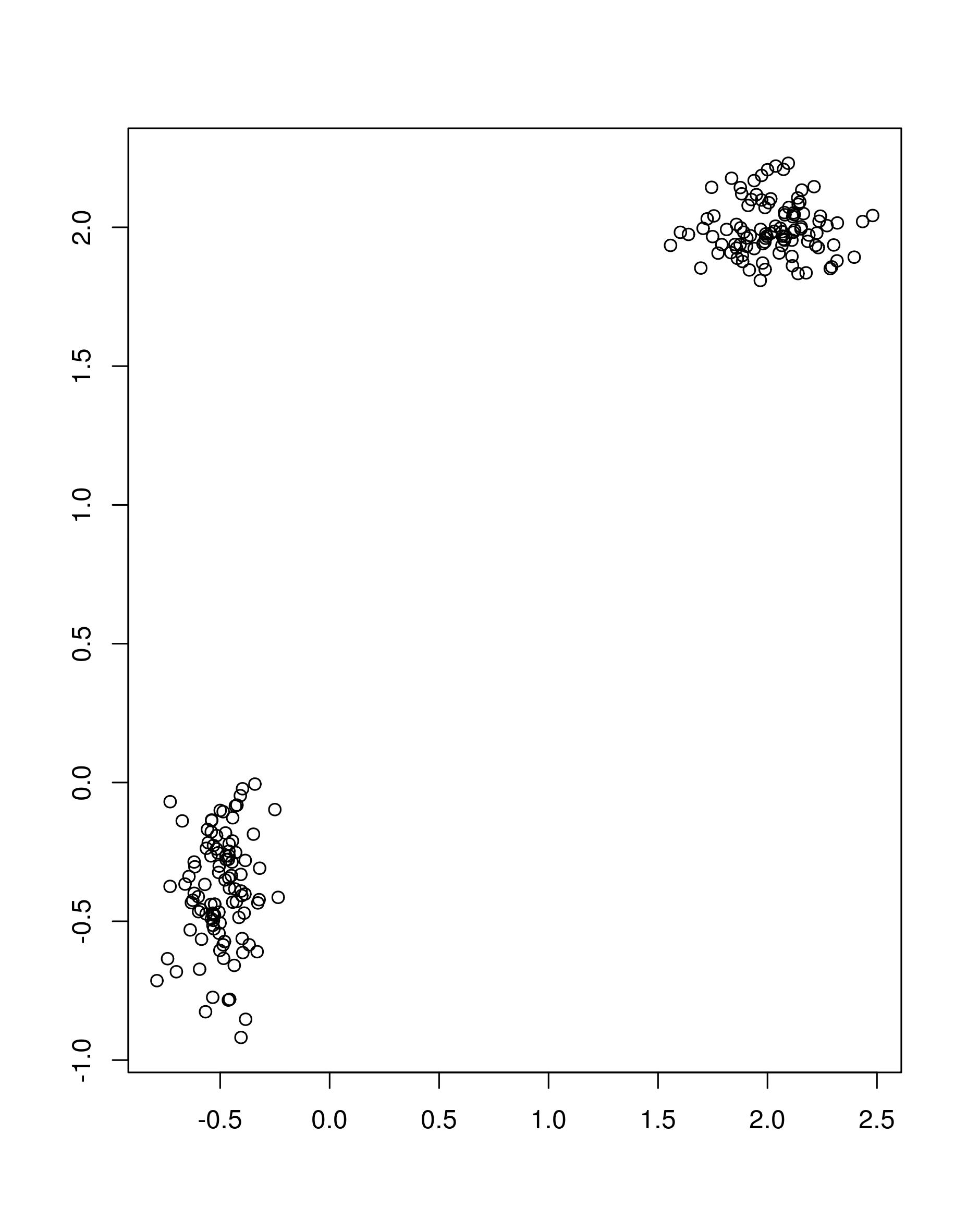
It is straightforward to use affinity propagation within R by simply using the function apcluster. First, we will create some toy data

set.seed(1)
cluster1 <- cbind(rnorm(100, 2, 0.2), rnorm(100, 2, 0.1))
cluster2 <- cbind(rnorm(100, -0.5, 0.1), rnorm(100, -0.4, 0.2))
mat <- rbind(cluster1, cluster2)

## visualize the two clusters
plot(mat, xlab = "", ylab = "")

In the next step, we apply the affinity progagation algorithm using the apcluster function. For the sake of demonstration, we will do this in two different ways that are however equivalent.

## alternative 1: apcluster computes the similarity matrix based on the input
## and the similarity function (here: negative square distances), 
## negDistMat(r = 2) refers here to standard similarity measure used in 
## Frey & Dueck (2007)
apc_1 <- apcluster(negDistMat(r = 2), mat)

## alternative 2: calculate first the similarity matrix based on the negative 
## square distances
mat_nd2 <- negDistMat(mat, r = 2)
apc_2 <- apcluster(mat_nd2)

By default, apcluster takes the median as the input preference (tendency of a data sample to become an exemplar). Adjusting this parameter (q) will increase (higher values of q) or decrease (lower values of q) the number of clusters returned by apcluster.

The APResult objects returned by apcluster contain information on the clustering result, including information on the total number of iterations, the sum of similarities, the sum of preferences, net similarity, the number of clusters and the cluster membership of the data points. The clusters can be accessed by apc_1@clusters, which will return a list containing the data points for the respective clusters. The apcluster allows to visualize the clustering result by entering

plot(apc_1, mat)

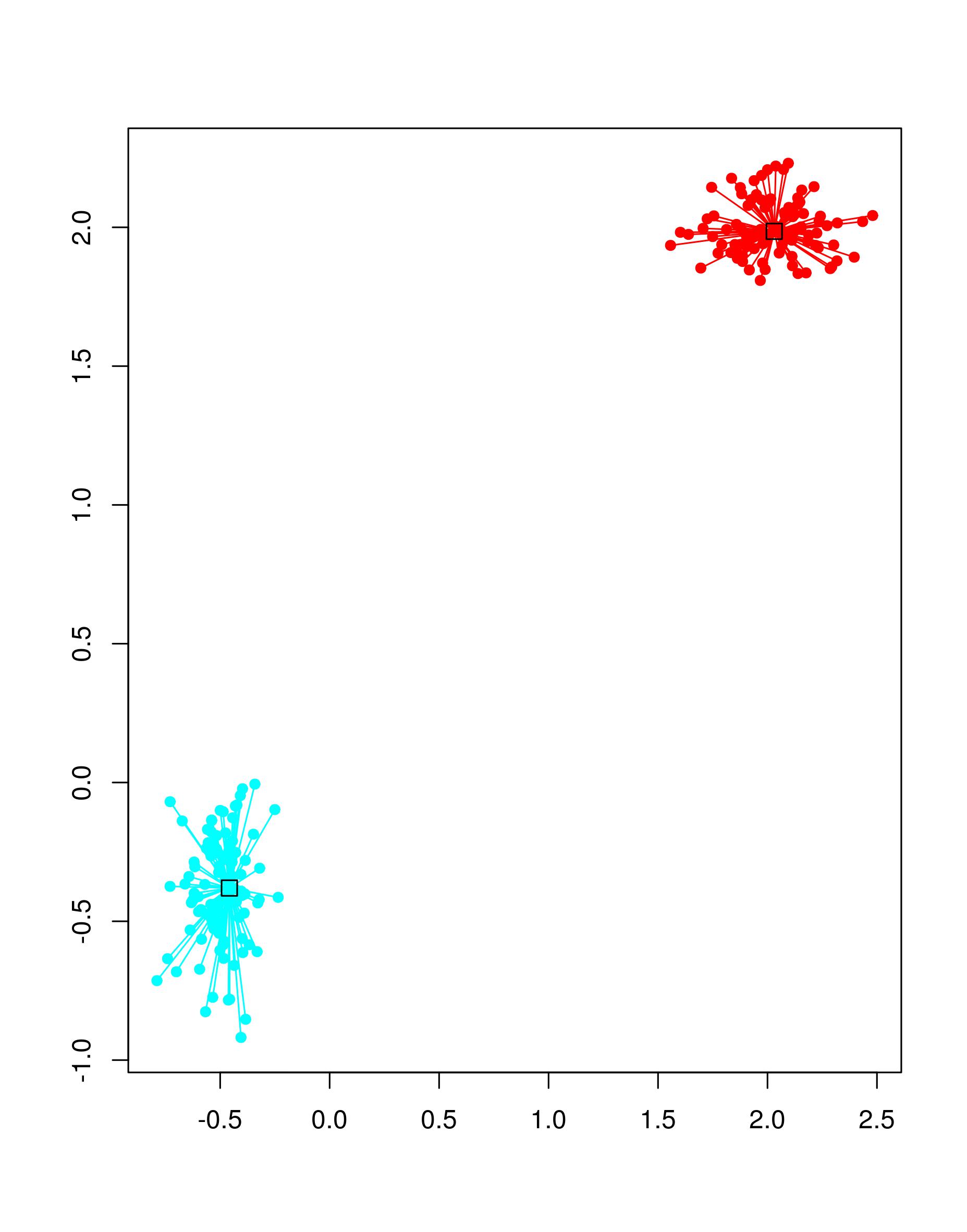
The two clusters are displayed in cyan and red; the two exemplars of the clusters are displayed as squares.

Several functions exist to analyze the output stored in the S4 object APResult returned by the function apcluster. The interested reader may consult the vignette of the apcluster package for further information on this topic.

The package also offers the possibility for exemplar-based agglomerative clustering (aggExCluster, merging of clusters is based on the identification of meaningful exemplars), leveraged affinity propagation (apclusterL, similarities of a subset of samples are used and different subsets of the data is used to iterativly improve the clustering result), and spare affinity propagation (apcluster, apclusterK = using a pre-defined number of clusters, using sparce matrices as defined by the Matrix package).

References

Frey B.J., Dueck D. Clustering by Passing Messages Between Data Points. Science, 315: 972-976, 2007, https://doi.org/10.1126/science.1136800

Bodenhofer U., Palme J., Melkonian C., Kothmeier A. APCluster - An R package for affinity propagation clustering